magrittr 管道操作

magrittr 相关文章收集

magrittr 管道操作能极大程度的简化数据处理，数据结构清晰明了

R语言中管道操作 %>%, %T>%, %$% 和 %<>%
magrittr 官方开发文档
 magrittr GitHub development page
and more…

magrittr - Ceci n’est pas un pipe

Description

The magrittr package offers a set of operators which promote semantics that will improve your code by

structuring sequences of data operations left-to-right (as opposed to from the inside and out)
avoiding nested function calls
minimizing the need for local variables and function definitions, and
making it easy to add steps anywhere in the sequence of operations.

The operators pipe their left-hand side values forward into expressions that appear on the right-hand side, i.e. one can replace f(x) with x %>% f, where %>% is the (main) pipe-operator.

Consider the example below. Four operations are performed to arrive at the desired data set, and they are written in a natural order: the same as the order of execution. Also, no temporary variables are needed. If yet another operation is required, it is straight-forward to add to the sequence of operations whereever it may be needed.

For a more detailed introduction see the vignette (vignette(“magrittr”)) or the documentation pages for the available operators:

%>%	 forward-pipe operator.
%T>%	 tee operator.
%<>%	 compound assignment pipe-operator.
%$%	 exposition pipe-operator.

Examples

## Not run: 

the_data <-
  read.csv('/path/to/data/file.csv') %>%
  subset(variable_a > x) %>%
  transform(variable_c = variable_a/veraiable_b) %>%
  head(100)

## End(Not run)

Introduction and basics

At first encounter, you may wonder whether an operator such as %>% can really be all that beneficial; but as you may notice, it semantically changes your code in a way that makes it more intuitive to both read and write.

Consider the following example, in which the mtcars dataset shipped with R is munged a little.

library(magrittr)
car_data <- 
  mtcars %>%
  subset(hp > 100) %>%
  aggregate(. ~ cyl, data = ., FUN = . %>% mean %>% round(2)) %>%
  transform(kpl = mpg %>% multiply_by(0.4251)) %>%
  print

  cyl   mpg   disp     hp drat   wt  qsec   vs   am gear carb       kpl
1   4 25.90 108.05 111.00 3.94 2.15 17.75 1.00 1.00 4.50 2.00 11.010090
2   6 19.74 183.31 122.29 3.59 3.12 17.98 0.57 0.43 3.86 3.43  8.391474
3   8 15.10 353.10 209.21 3.23 4.00 16.77 0.00 0.14 3.29 3.50  6.419010

We start with a value, here mtcars (a data.frame). Based on this, we first extract a subset, then we aggregate the information based on the number of cylinders, and then we transform the dataset by adding a variable for kilometers per liter as supplement to miles per gallon. Finally we print the result before assigning it. Note how the code is arranged in the logical order of how you think about the task: data->transform->aggregate, which is also the same order as the code will execute. It’s like a recipe – easy to read, easy to follow!

A horrific alternative would be to write

car_data <- transform(aggregate(. ~ cyl, 
                      data = subset(mtcars, hp > 100), 
                      FUN = function(x) round(mean(x, 2))), 
                      kpl = mpg*0.4251)

There is a lot more clutter with parentheses, and the mental task of deciphering the code is more challenging—in particular if you did not write it yourself.

Note also how “building” a function on the fly for use in aggregate is very simple in magrittr: rather than an actual value as left-hand side in pipeline, just use the placeholder. This is also very useful in R’s *apply family of functions.

Granted: you may make the second example better, perhaps throw in a few temporary variables (which is often avoided to some degree when using magrittr), but one often sees cluttered lines like the ones presented.

And here is another selling point. Suppose I want to quickly want to add another step somewhere in the process. This is very easy in the to do in the pipeline version, but a little more challenging in the “standard” example.

The combined example shows a few neat features of the pipe (which it is not):

By default the left-hand side (LHS) will be piped in as the first argument of the function appearing on the right-hand side (RHS). This is the case in the subset and transform expressions.
%>% may be used in a nested fashion, e.g. it may appear in expressions within arguments. This is used in the mpg to kpl conversion.
When the LHS is needed at a position other than the first, one can use the dot,’.’, as placeholder. This is used in the aggregate expression.
The dot in e.g. a formula is not confused with a placeholder, which is utilized in the aggregate expression.
Whenever only one argument is needed, the LHS, then one can omit the empty parentheses. This is used in the call to print (which also returns its argument). Here, LHS %>% print(), or even LHS %>% print(.) would also work.
A pipeline with a dot (.) as LHS will create a unary function. This is used to define the aggregator function.

One feature, which was not utilized above is piping into anonymous functions, or lambdas. This is possible using standard function definitions, e.g.

car_data %>%
  (function(x) {
    if (nrow(x) > 2) 
      rbind(head(x, 1), tail(x, 1))
    else x
  })

1
2
3

  cyl mpg disp  hp drat wt qsec vs am gear carb     kpl
1   4  26  108 111    4  2   18  1  1    4    2 11.0526
3   8  15  350 192    3  4   17  0  0    3    4  6.3765

However, magrittr also allows a short-hand notation:

car_data %>%
{ 
  if (nrow(.) > 0)
    rbind(head(., 1), tail(., 1))
  else .
}

1
2
3

  cyl mpg disp  hp drat wt qsec vs am gear carb     kpl
1   4  26  108 111    4  2   18  1  1    4    2 11.0526
3   8  15  350 192    3  4   17  0  0    3    4  6.3765

Since all right-hand sides are really “body expressions” of unary functions, this is only the natural extension the simple right-hand side expressions. Of course longer and more complex functions can be made using this approach.

In the first example the anonymous function is enclosed in parentheses. Whenever you want to use a function- or call-generating statement as right-hand side, parentheses are used to evaluate the right-hand side before piping takes place.

Another, less useful example is:

1	1:10 %>% (substitute(f(), list(f = sum)))

[1] 55

Additional pipe operators

magrittr also provides three related pipe operators. These are not as common as %>% but they become useful in special cases.

The “tee” operator, %T>% works like %>%, except it returns the left-hand side value, and not the result of the right-hand side operation. This is useful when a step in a pipeline is used for its side-effect (printing, plotting, logging, etc.). As an example (where the actual plot is omitted here):

rnorm(200) %>%
matrix(ncol = 2) %T>%
plot %>% # plot usually does not return anything. 
colSums

1	[1] -4.835279 -5.274882

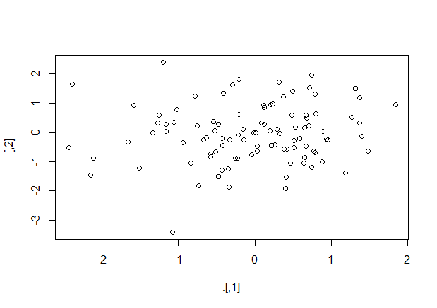
The “exposition” pipe operator, %$% exposes the names within the left-hand side object to the right-hand side expression. Essentially, it is a short-hand for using the with functions (and the same left-hand side objects are accepted). This operator is handy when functions do not themselves have a data argument, as for example lm and aggregate do. Here are a few examples as illustration:

iris %>%
  subset(Sepal.Length > mean(Sepal.Length)) %$%
  cor(Sepal.Length, Sepal.Width)

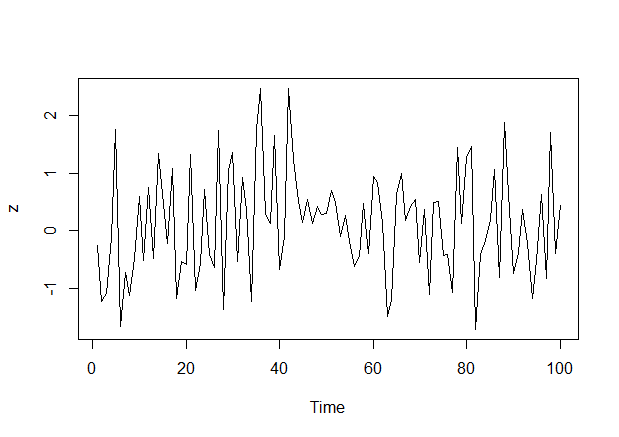
data.frame(z = rnorm(100)) %$% 
  ts.plot(z)

1	[1] 0.3361992

Finally, the compound assignment pipe operator %<>% can be used as the first pipe in a chain. The effect will be that the result of the pipeline is assigned to the left-hand side object, rather than returning the result as usual. It is essentially shorthand notation for expressions like foo <- foo="" %="">% bar %>% baz, which boils down to foo %<>% bar %>% baz. Another example is

1	iris$Sepal.Length %<>% sqrt

The %<>% can be used whenever expr <- … makes sense, e.g.

x %<>% foo %>% bar
x[1:10] %<>% foo %>% bar
x$baz %<>% foo %>% bar

Aliases

In addition to the %>%-operator, magrittr provides some aliases for other operators which make operations such as addition or multiplication fit well into the magrittr-syntax. As an example, consider:

rnorm(1000)    %>%
  multiply_by(5) %>%
  add(5)         %>%
  { 
    cat("Mean:", mean(.), 
        "Variance:", var(.), "\n")
    head(.)
  }

1 2	Mean: 4.912365 Variance: 24.46778 [1] 5.853147 3.923652 7.802787 10.208513 2.239128 3.177795

which could be written in more compact form as

rnorm(100) %>% `*`(5) %>% `+`(5) %>% 
{
  cat("Mean:", mean(.), "Variance:", var(.),  "\n")
  head(.)
}

1 2	Mean: 5.443435 Variance: 30.92747 [1] 2.7712630 1.9156065 2.9230592 7.8741192 3.2132655 0.1729982

To see a list of the aliases, execute e.g. ?multiply_by.