1 | library(lattice) |
之前制作的 Power BI 文件都放在 GitHub 里面,可操作性差
点击 超链接 进入 GitHub → 选择文件下载 → 本地打开
竟然如此麻烦,还是看看效果图片就好

现在!
没错,就是现在!
可以网页一步到位,power bi web 共享了解一下?

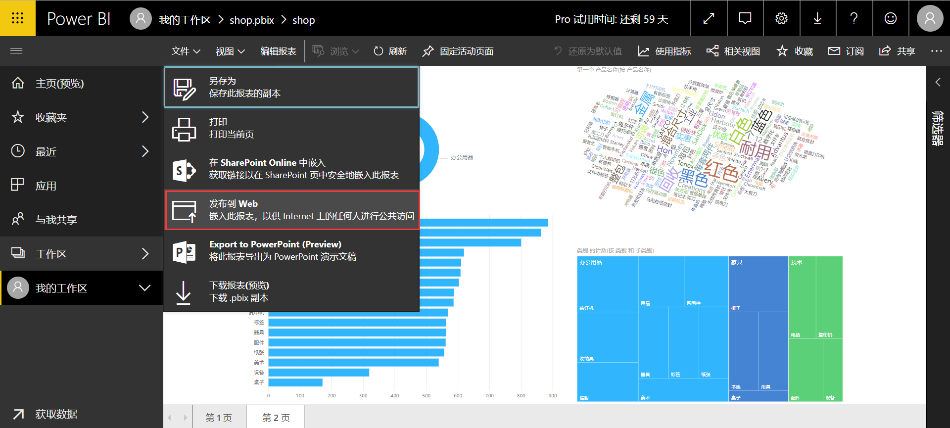

power bi pro 可以实现 web 共享,免费试用60天


magrittr 管道操作能极大程度的简化数据处理,数据结构清晰明了
R语言中管道操作 %>%, %T>%, %$% 和 %<>%
magrittr 官方开发文档
magrittr GitHub development page
and more…
The magrittr package offers a set of operators which promote semantics that will improve your code by
The operators pipe their left-hand side values forward into expressions that appear on the right-hand side, i.e. one can replace f(x) with x %>% f, where %>% is the (main) pipe-operator.
Consider the example below. Four operations are performed to arrive at the desired data set, and they are written in a natural order: the same as the order of execution. Also, no temporary variables are needed. If yet another operation is required, it is straight-forward to add to the sequence of operations whereever it may be needed.
For a more detailed introduction see the vignette (vignette(“magrittr”)) or the documentation pages for the available operators:1
2
3
4%>% forward-pipe operator.
%T>% tee operator.
%<>% compound assignment pipe-operator.
%$% exposition pipe-operator.
1 | ## Not run: |
At first encounter, you may wonder whether an operator such as %>% can really be all that beneficial; but as you may notice, it semantically changes your code in a way that makes it more intuitive to both read and write.
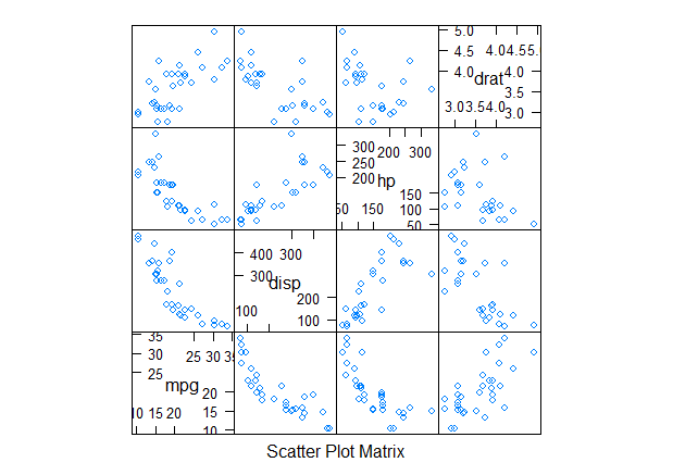
Consider the following example, in which the mtcars dataset shipped with R is munged a little.
1 | library(magrittr) |
1 | cyl mpg disp hp drat wt qsec vs am gear carb kpl |
We start with a value, here mtcars (a data.frame). Based on this, we first extract a subset, then we aggregate the information based on the number of cylinders, and then we transform the dataset by adding a variable for kilometers per liter as supplement to miles per gallon. Finally we print the result before assigning it. Note how the code is arranged in the logical order of how you think about the task: data->transform->aggregate, which is also the same order as the code will execute. It’s like a recipe – easy to read, easy to follow!
A horrific alternative would be to write1
2
3
4car_data <- transform(aggregate(. ~ cyl,
data = subset(mtcars, hp > 100),
FUN = function(x) round(mean(x, 2))),
kpl = mpg*0.4251)
There is a lot more clutter with parentheses, and the mental task of deciphering the code is more challenging—in particular if you did not write it yourself.
Note also how “building” a function on the fly for use in aggregate is very simple in magrittr: rather than an actual value as left-hand side in pipeline, just use the placeholder. This is also very useful in R’s *apply family of functions.
Granted: you may make the second example better, perhaps throw in a few temporary variables (which is often avoided to some degree when using magrittr), but one often sees cluttered lines like the ones presented.
And here is another selling point. Suppose I want to quickly want to add another step somewhere in the process. This is very easy in the to do in the pipeline version, but a little more challenging in the “standard” example.
The combined example shows a few neat features of the pipe (which it is not):
One feature, which was not utilized above is piping into anonymous functions, or lambdas. This is possible using standard function definitions, e.g.1
2
3
4
5
6car_data %>%
(function(x) {
if (nrow(x) > 2)
rbind(head(x, 1), tail(x, 1))
else x
})
1 | cyl mpg disp hp drat wt qsec vs am gear carb kpl |
However, magrittr also allows a short-hand notation:1
2
3
4
5
6car_data %>%
{
if (nrow(.) > 0)
rbind(head(., 1), tail(., 1))
else .
}
1 | cyl mpg disp hp drat wt qsec vs am gear carb kpl |
Since all right-hand sides are really “body expressions” of unary functions, this is only the natural extension the simple right-hand side expressions. Of course longer and more complex functions can be made using this approach.
In the first example the anonymous function is enclosed in parentheses. Whenever you want to use a function- or call-generating statement as right-hand side, parentheses are used to evaluate the right-hand side before piping takes place.
Another, less useful example is:1
1:10 %>% (substitute(f(), list(f = sum)))
1 | [1] 55 |
magrittr also provides three related pipe operators. These are not as common as %>% but they become useful in special cases.
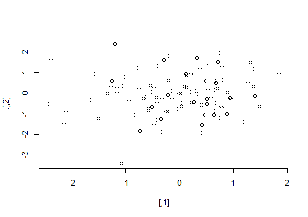
The “tee” operator, %T>% works like %>%, except it returns the left-hand side value, and not the result of the right-hand side operation. This is useful when a step in a pipeline is used for its side-effect (printing, plotting, logging, etc.). As an example (where the actual plot is omitted here):
1 | rnorm(200) %>% |
1 | [1] -4.835279 -5.274882 |
The “exposition” pipe operator, %$% exposes the names within the left-hand side object to the right-hand side expression. Essentially, it is a short-hand for using the with functions (and the same left-hand side objects are accepted). This operator is handy when functions do not themselves have a data argument, as for example lm and aggregate do. Here are a few examples as illustration:1
2
3
4
5
6iris %>%
subset(Sepal.Length > mean(Sepal.Length)) %$%
cor(Sepal.Length, Sepal.Width)
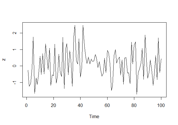
data.frame(z = rnorm(100)) %$%
ts.plot(z)
1 | [1] 0.3361992 |
Finally, the compound assignment pipe operator %<>% can be used as the first pipe in a chain. The effect will be that the result of the pipeline is assigned to the left-hand side object, rather than returning the result as usual. It is essentially shorthand notation for expressions like foo <- foo="" %="">% bar %>% baz, which boils down to foo %<>% bar %>% baz. Another example is1
iris$Sepal.Length %<>% sqrt
The %<>% can be used whenever expr <- … makes sense, e.g.
In addition to the %>%-operator, magrittr provides some aliases for other operators which make operations such as addition or multiplication fit well into the magrittr-syntax. As an example, consider:1
2
3
4
5
6
7
8rnorm(1000) %>%
multiply_by(5) %>%
add(5) %>%
{
cat("Mean:", mean(.),
"Variance:", var(.), "\n")
head(.)
}
1 | Mean: 4.912365 Variance: 24.46778 |
which could be written in more compact form as1
2
3
4
5rnorm(100) %>% `*`(5) %>% `+`(5) %>%
{
cat("Mean:", mean(.), "Variance:", var(.), "\n")
head(.)
}
1 | Mean: 5.443435 Variance: 30.92747 |
To see a list of the aliases, execute e.g. ?multiply_by.
通用代码1
<iframe height=400 width=700 src='http://music.163.com/m/mv?id=10770095&userid=340573904' frameborder=0 'allowfullscreen'></iframe>
修改的src后的链接即可
如果需要在表格或区域中按行查找内容,可使用 VLOOKUP,它是一个查找和引用函数。例如,按部件号查找汽车部件的价格。
在这一最简单的形式中,VLOOKUP 函数表示:
=VLOOKUP(要查找的值、要在其中查找值的区域、区域中包含返回值的列号、精确匹配或近似匹配 – 指定为 0/FALSE 或 1/TRUE)。
使用 VLOOKUP 函数在表中查找值。
语法
VLOOKUP (lookup_value, table_array, col_index_num, [range_lookup])
例如:
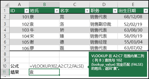
=VLOOKUP(105,A2:C7,2,TRUE)
=VLOOKUP(“袁”,B2:E7,2,FALSE)
| 参数名称 | 说明 |
|---|---|
| lookup_value (必需参数) | 要查找的值。要查找的值必须位于 table-array 中指定的单元格区域的第一列中。 |
| 例如,如果 table-array 指定的单元格为 B2:D7,则 lookup_value 必须位于列 B 中。请参见下图。Lookup_value 可以是值,也可以是单元格引用。 | |
| Table_array (必需参数) | VLOOKUP 在其中搜索 lookup_value 和返回值的单元格区域。 |
| 该单元格区域中的第一列必须包含 lookup_value(例如,下图中的“姓氏”)。此单元格区域中还需要包含您要查找的返回值(例如,下图中的“名字”)。 | |
| 了解如何选择工作表中的区域。 | |
| col_index_num (必需参数) | 其中包含返回值的单元格的编号(table-array 最左侧单元格为 1 开始编号)。 |
| range_lookup (可选参数) | 一个逻辑值,该值指定希望 VLOOKUP 查找近似匹配还是精确匹配: |
| TRUE 假定表中的第一列按数字或字母排序,然后搜索最接近的值。这是未指定值时的默认方法。 | |
| FALSE 在第一列中搜索精确值。 |
需要四条信息才能构建 VLOOKUP 语法:
1、要查找的值,也被称为查阅值。
2、查阅值所在的区域。请记住,查阅值应该始终位于所在区域的第一列,这样 VLOOKUP 才能正常工作。例如,如果查阅值位于单元格 C2 内,那么您的区域应该以 C 开头。
3、区域中包含返回值的列号。例如,如果指定 B2:D11 作为区域,那么应该将 B 算作第一列,C 作为第二列,以此类推。
4、(可选)如果需要返回值的近似匹配,可以指定 TRUE;如果需要返回值的精确匹配,则指定 FALSE。如果没有指定任何内容,默认值将始终为 TRUE 或近似匹配。
现在将上述所有内容集中在一起,如下所示:
=VLOOKUP(查阅值、包含查阅值的区域、区域中包含返回值的列号以及(可选)为近似匹配指定 TRUE 或者为精确匹配指定 FALSE)。
例如: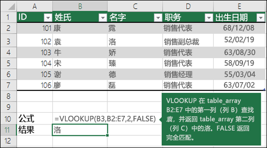
文章来源:excel官方文档
作者介绍:皮吉斯,热爱R语言,知乎号:皮吉斯
已授权转载
本次的分析数据来自kaggle数据竞赛平台的 “give me some credit” 竞赛项目。任务是提高模型精度AUC。
本次分析用到了多种算法,分别有:逻辑回归,cart决策树,神经网络,xgboost,随机森林。通过多种模型相互对比,最终根据auc选出最好的模型。
1 | cs_training <- read.csv("cs_training.csv") |
导入数据,并对列名重命名,方便分析。
通过summary了解数据的整体情况,可以看到monthliincome和x7变量有缺失值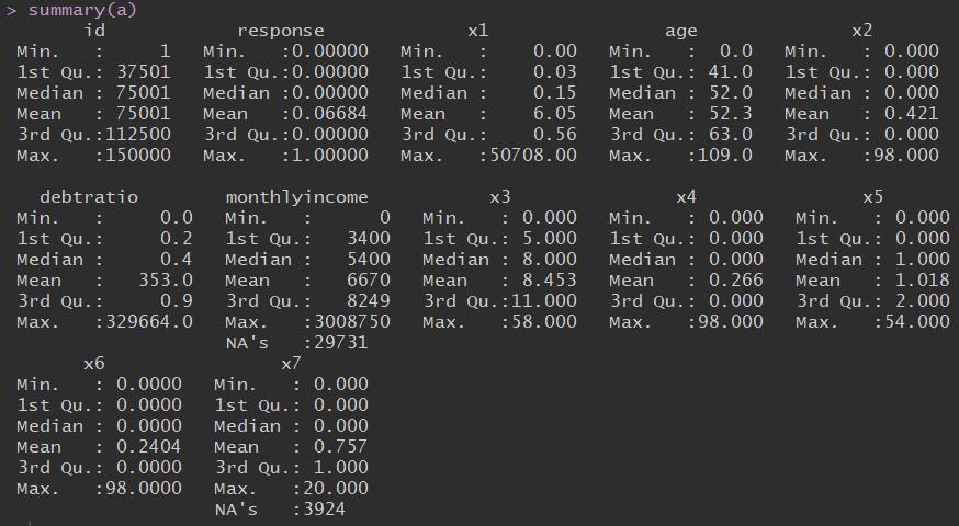
1 | #age变量 |
| var | mean | median | 0 | 0.01 | 0.1 | 0.25 | 0.5 | 0.75 | 0.9 | 0.99 | 1 | max | missing |
|---|---|---|---|---|---|---|---|---|---|---|---|---|---|
| age | 52.2952066666667 | 52 | 0 | 24 | 33 | 41 | 52 | 63 | 72 | 87 | 109 | 109 | 0 |
这样可以看到各个变量的数据分布情况1
2# 查看异常值
boxplot(age~response,data = a,horizontal = T ,frame = F , col = "lightgray",main = "Distribution")
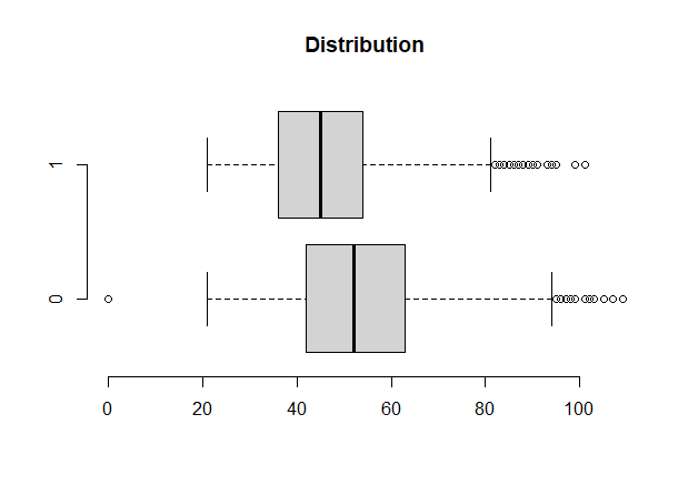
上图可以看到,数据存在异常值。
处理异常值:通常采用盖帽法,即用数据分布在1%的数据覆盖在1%以下的数据,用在99%的数据覆盖99%以上的数据。1
2
3
4
5
6
7
8
9
10
11
12block<-function(x,lower=T,upper=T){
if(lower){
q1<-quantile(x,0.01)
x[x<=q1]<-q1
}
if(upper){
q99<-quantile(x,0.99)
x[x>q99]<-q99
}
return(x)
}
boxplot(age~response,data = a,horizontal = T ,frame = F , col = "lightgray",main = "Distribution")
经过处理,异常值大量减少1
2
3
4
5
6
7
8
9
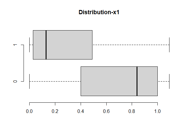
10# x1
xa1<-a$x1
var_x1<-c(var='xa1',
mean=mean(xa1,na.rm = T),
median=median(xa1,na.rm = T),
quantile(xa1,c(0,0.01,0.1,0.5,0.75,0.9,0.99,1),na.rm = T), max=max(xa1,na.rm = T),
miss=sum(is.na(xa1)) )
boxplot(x1~response,data=a,horizontal=T, frame=F, col="lightgray",main="Distribution-x1")
#对X1变量进行处理
a$x1<-block(a$x1)
1
2
3
4
5
6
7
8
9
10
11
12
13
14
15
16
17
18
19
20
21
22
23
24
25
26
27
28
29
30
31
32
33
34
35
36
37
38# x2
a$x2
summary(a$x2)
xa2<-a$x2
var_x2<-c(var='xa2',
mean=mean(xa2,na.rm = T),
median=median(xa2,na.rm = T),
quantile(xa2,c(0,0.01,0.1,0.5,0.75,0.9,0.99,1),na.rm = T), max=max(xa2,na.rm = T),
miss=sum(is.na(xa2)) )
boxplot(x2~response,data=a,horizontal=T, frame=F, col="lightgray",main="Distribution")
# 对x2变量进行处理
a$x2<-block(a$x2)
a$x1<-round(a$x1,2)
# debtratio
summary(a$debtratio)
ratio<-a$debtratio
var_ratio<-c(var='debtratio',
mean=mean(ratio,na.rm = T),
median=median(ratio,na.rm = T),
quantile(ratio,c(0,0.01,0.1,0.5,0.75,0.9,0.99,1),na.rm = T), max=max(ratio,na.rm = T),
miss=sum(is.na(ratio)) )
hist(a$debtratio)
# 因为debtratio是百分比,对异常值的处理要结合实际
a$debtratio<-ifelse(a$debtratio>1,1,a$debtratio)
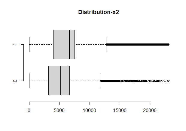
# monthlyincome
income<-a$monthlyincome
var_income<-c(var='income',
mean=mean(income,na.rm = T),
median=median(income,na.rm = T),
quantile(income,c(0,0.01,0.1,0.5,0.75,0.9,0.99,1),na.rm = T),
max=max(income,na.rm = T),
miss=sum(is.na(income)) )
hist(income)
boxplot(monthlyincome~response,data=a,horizontal=T, frame=F, col="lightgray",main="Distribution-x2")
# 对缺失值处理
a$monthlyincome<-ifelse(is.na(a$monthlyincome)==T,6670.2,a$monthlyincome)
# 对异常值处理
a$monthlyincome<-block(a$monthlyincome)
1
2
3
4
5
6
7
8
9
10# x3
summary(a$x3)
x3<-a$x3
var_x3<-c(var='x3',mean=mean(x3,na.rm = T),
median=median(x3,na.rm = T),
quantile(x3,c(0,0.01,0.1,0.5,0.75,0.9,0.99,1),na.rm = T), max=max(x3,na.rm = T),
miss=sum(is.na(x3)) )
names(a)
# 对x3进行处理
a$x3<-block(a$x3)
1 | # x4-延迟90天的次数 |
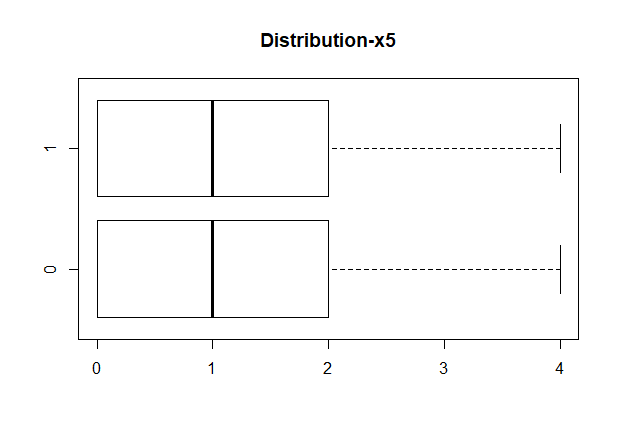
1 | # x5-贷款额度 |
1
2
3
4
5
6
7
8
9# x6
summary(a$x6)
x6<-a$x6
var_x6<-c(var='x6',mean=mean(x6,na.rm = T),
median=median(x6,na.rm = T),
quantile(x6,c(0,0.01,0.1,0.5,0.75,0.9,0.99,1),na.rm = T), max=max(x6,na.rm = T),
miss=sum(is.na(x6)) )
# 对x6进行盖帽法
a$x6<-block(a$x6)
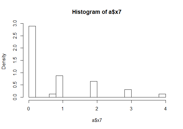
1 | # x7 |
1
2
3#response变量
# 为了方便理解,将1作为违约,0表示不违约
a$response<-as.numeric(!as.logical(a$response))
1 | table(a$response) |
| 0 | 1 |
| 10026 | 139974 |
数据正负比例不平衡,我们要对数据进行smote处理,smote算法的思想是合成新的少数类样本,合成的策略是对每个少数类样本a,从它的最近邻中随机选一个样本b,然后在a、b之间的连线上随机选一点作为新合成的少数类样本。
1 | library(lattice) |
1 | # 接下来进行分组 |
table(train$response)
| 0 | 1 |
| 21213 | 27914 |
table(test$response)
| 0 | 1 |
| 8865 | 12190 |
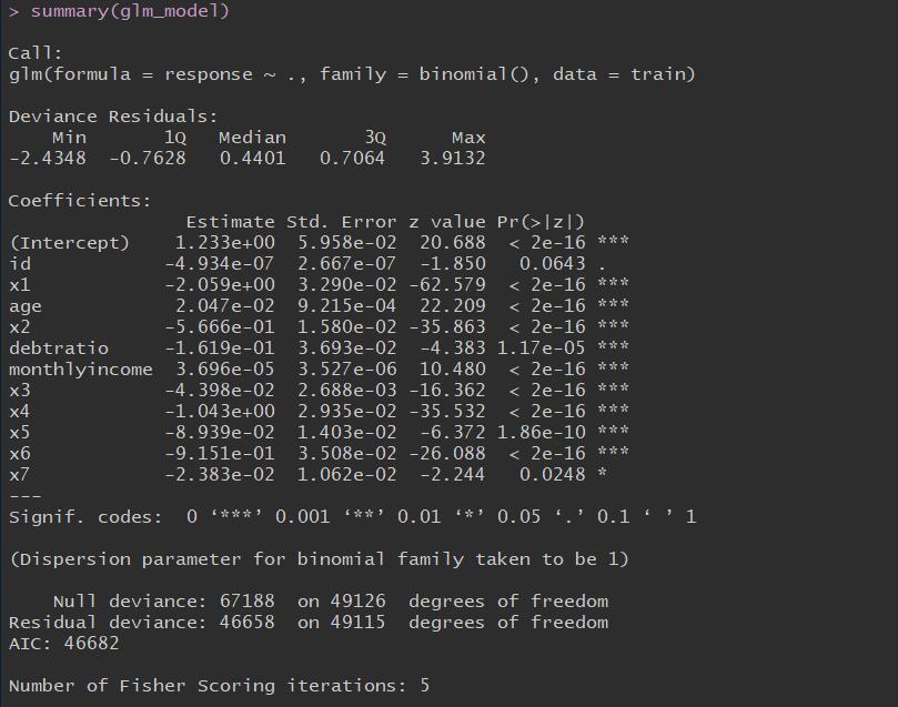
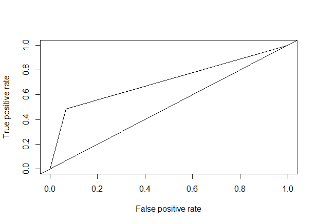
1 | glm_model <- glm(response~. , data = train , family = binomial()) |
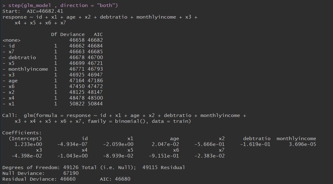
1 | step(glm_model , direction = "both") |
1 | library(carData) |

1 | train_pred <- predict(glm_model , newdata = train , type = "response") |
1 | library(gplots) |
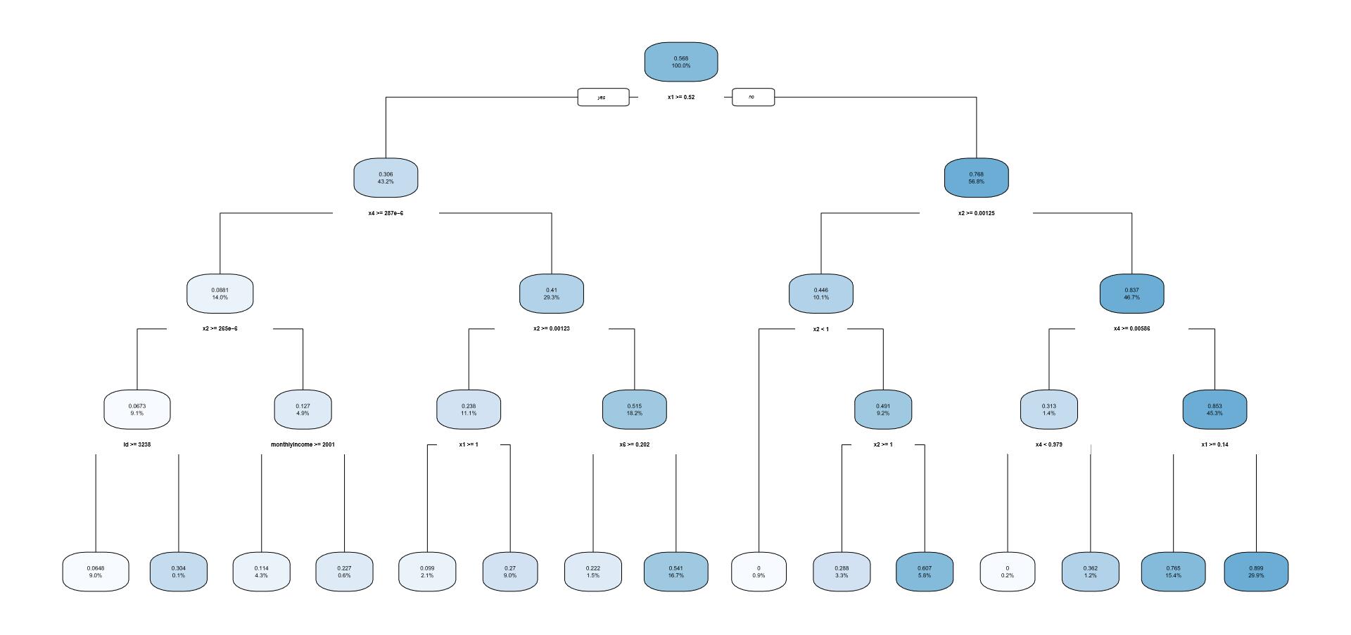
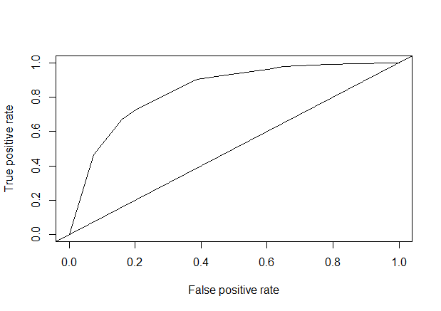
1 | library(rpart) |
1 | test_pred <- predict(cart_model , newdata = test) |
1 | test_prob <- prediction(test_pred, test$response) |
1 | #对数据进行标准化 |
1 | library(nnet) |
1 | test_pred<-predict(train_nnet, test) |
test_pred
| 0 | 1 |
| 14523 | 6532 |
1 | test_pred_rate<-sum(test_pred==test$response)/length(test$response) |
1 | library(gplots) |
1 | ##输入数据的预测变量必须是二分类的。且所有变量只包含模型输入输出变量。 |
1 | #调参后的模型 #size =11 , decay = 0.0013 , maxit = 200 |
1 | # 预测为0,1 |
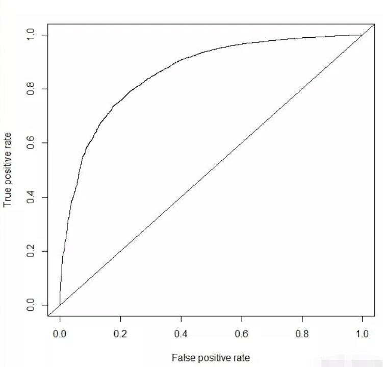
1 | library(xgboost) |
1 | test_prob <- predict(xgb_model , data.matrix(test[,-1])) |
1 | test_pred <- prediction(test_prob , test$response) |
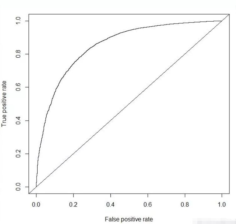
1 | library(randomForest) |
1 | test_prob <- predict(random_model , test , type= "response") |
1 | test_pred <- prediction(test_prob , test$response) |
综上,通过多种模型对比可以看到xgboost算法的模型精确度是最高的达到0.860617。